4.6. An Empirical Analysis under Multiple Models

For this tutorial, I will assume that you have already run through the simple empirical analysis, so we will go into a lot less detail here.

In the tutorial for the simple empirical analysis, we performed a basic analysis of the lizard sequence data under the model specified in the dpp-simple.cfg configuration file. We did this by entering the following at the command line from within the pymsbayes-tutorial-data/lizards/configs directory:

$ dmc.py -o dpp-simple.cfg -p dpp-simple.cfg -n 5000

One nice feature of dmc.py is that it is very easy to perform analyses of the same data under an arbitrary number of different models. For example, we can easily expand on our example above to analyze the lizard data under two different models: the dpp-msbayes model specified in the pymsbayes-tutorial-data/lizards/configs/dpp-simple.cfg configuration file and an msBayes model specified in the pymsbayes-tutorial-data/lizards/configsmsbayes.cfg file:

$ dmc.py -o dpp-simple.cfg -p dpp-simple.cfg msbayes.cfg -n 5000

Notice, we now specify both of the model configuration files for the prior model (-p) option. Also, because both of the configuration files share the same sample table, it does not matter which one is specified for the observed-data configuration option (-o) (i.e., either way the observed summary statistics will be calculated from the same sequence alignments).

What this new command accomplishes is that dmc.py will now analyze the data under both models simultaneously. This will take a little longer to run than the previous analysis, but should finish in less than a few minutes or so on a modern laptop.

The msbayes.cfg configuration file has the following preamble:

lowerTheta = 0.0
upperTheta = 0.01
timeInSubsPerSite = 1
lowerTau = 0.0
upperTau = 0.1
numTauClasses = 0
upperMig = 0.0
upperRec = 0.0
upperAncPopSize = 1.0

This specifies an msBayes model that is roughly equivalent to the dpp-msbayes model specified in dpp-simple.cfg in terms of prior uncertainty about divergence times and population sizes. Notice that PyMsBayes and the version of msBayes that comes with dpp-msbayes support the options lowerTau and timeInSubsPerSite, which are not supported in the msBayes version of [6].

4.6.1. The output

Because we analyzed the data under two models, we will now have more output. There should be a new directory named pymsbayes-results that was created when you ran the analysis. If you still had the pymsbayes-results in the pymsbayes-tutorial-data/lizards/configs from the previous analysis, then the new results will be output to a new directory named pymsbayes-results-0.

4.6.1.1. The info file

Our new pymsbayes-results/pymsbayes.info.txt, will look something like:

[pymsbayes]
    version = Version 0.2.4
    output_directory = /home/jamie/software/dev/pymsbayes-tutorial-data/lizards/configs/pymsbayes-results-0
    temp_directory = /home/jamie/software/dev/pymsbayes-tutorial-data/lizards/configs/pymsbayes-results-0/temp-files-5ym88h
    sort_index = 0
    simulation_reps = 0
    seed = 192883961
    num_processors = 8
    num_prior_samples = 5000
    num_standardizing_samples = 5000
    bandwidth = 0.002
    posterior_quantiles = 1000
    posterior_sample_size = 1000
    stat_patterns = ^\s*pi\.\d+\s*$, ^\s*wattTheta\.\d+\s*$, ^\s*pi\.net\.\d+\s*$, ^\s*tajD\.denom\.\d+\s*$
    num_taxon_pairs = 3
    dry_run = False
    [[tool_paths]]
            dpp_msbayes = /home/jamie/software/dev/PyMsBayes/bin/linux/dpp-msbayes.pl
            msbayes = /home/jamie/software/dev/PyMsBayes/bin/linux/msbayes.pl
            eureject = /home/jamie/software/dev/PyMsBayes/bin/linux/eureject
            abcestimator = /home/jamie/software/dev/PyMsBayes/bin/linux/ABCestimator
    [[observed_configs]]
            1 = ../dpp-simple.cfg
    [[observed_paths]]
            1 = observed-summary-stats/observed-1.txt
    [[prior_configs]]
            1 = ../dpp-simple.cfg
            2 = ../msbayes.cfg
    [[run_stats]]
            start_time = 2015-02-11 19:40:17.874783
            stop_time = 2015-02-11 19:41:33.645795
            total_duration = 0:01:15.771012

This is very similar to our first analysis, except that there are now two prior configs listed.

4.6.1.2. The data and model keys and corresponding directories

If we look within the new pymsbayes-results/pymsbayes-output directory, we will see that the model-key.txt now contains:

m1 = ../../dpp-simple.cfg
m2 = ../../msbayes.cfg

This tells us that we will find the results of the analysis under the dpp-simple.cfg model within the pymsbayes-results/pymsbayes-output/d1/m1 directory, and will find the results of the analysis under the msbayes.cfg model within the pymsbayes-results/pymsbayes-output/d1/m2 directory.

4.6.1.3. Model-averaged results

In addition to the results of the analyses under both models, there are also results in the pymsbayes-results/pymsbayes-output/d1/m12-combined directory that are averaged over both models. This kind of model-averaging analysis was encouraged by [5], however, [9] found such model-averaged analyses to perform quite poorly. Nonetheless, the option is yours to explore these types of model-averaging analyses.

Rather than summarize and plot the results of this very short example multi-model analysis, let’s go ahead and look at some output from the same analysis run for many more samples from the priors.

4.6.2. Output from a longer analysis

In the tutorial data you downloaded, you can find the output of the same multi-model analysis we ran above, but run for much longer. You can find these results in the directory, pymsbayes-tutorial-data/lizards/results/sample-output/lizard-analysis.

These results were generated via the following command, which took less than a day to run on a laptop:

$ dmc.py --np 8 \
    -o dpp-simple.cfg \
    -p dpp-simple.cfg msbayes.cfg \
    -n 10000000 \
    --prior-batch-size 12500 \
    --num-posterior-samples 1000 \
    --num-standardizing-samples 100000 \
    -q 1000 \
    --reporting-frequency 200000 \
    --compress \
    --seed 845225390

You can see the full bash script that was used to run this analysis in the file pymsbayes-tutorial-data/lizards/bin/example-qsub.sh. We can see that this analysis will draw 10 million samples from both prior models (-n 10000000), and report the results every 200,000 samples (--reporting-frequency 200000). Furthermore, the first 100,000 samples from each prior will be used to standardize the summary statistics calculated from all the prior simulations and the observed data (--num-standardizing-samples 100000). I chose the number of processes (--np 8) and the size of the “batches” in which the prior samples will be generated (--prior-batch-size 12500) such that their product (100,000 samples) is a common factor of the number of standardizing samples (100,000), the reporting frequency (200,000), and the total number of samples (10 million). This is not mandatory, but it will maximize the efficiency of the multi-processing. I also specify a seed for the random number generator (--seed 845225390) so that I, or anyone else, can replicate the results. The seed is always reported in the pymsbayes-info.txt file, so this is not necessary unless you are trying to replicate previous results. But, it is always good to report the seed (or at least make it available) so that others can replicate your work.

4.6.2.1. Additional results reported during analysis

If we look in the pymsbayes-tutorial-data/lizards/results/sample-output/lizard-analysis/pymsbayes-results directory, we will find that most of the output (e.g., the info file, key files, directory structure) is very similar to the short analysis we ran above. The main difference is in the number of result files that are in the pymsbayes-tutorial-data/lizards/results/sample-output/lizard-analysis/pymsbayes-results/pymsbayes-output/d1/m1 , pymsbayes-tutorial-data/lizards/results/sample-output/lizard-analysis/pymsbayes-results/pymsbayes-output/d1/m2 , and pymsbayes-tutorial-data/lizards/results/sample-output/lizard-analysis/pymsbayes-results/pymsbayes-output/d1/m12-combined directories. As you can see, we have results files for every 200,000 prior samples.

4.6.2.2. The trace file

There is also an additional “trace” file:

• d1-m1-s1-trace.txt

Which shows the posterior means of various estimates as the prior samples accumulated. This file is created whenever the --reporting-frequency option is used to report results as the analysis progresses. This file is useful for checking to see if estimates stabilized as the number of prior samples evaluated increased, and to see if estimates from multiple, independent analyses “converged” to similar estimates.

4.6.2.3. Plotting the results

Go ahead and navigate into the pymsbayes-tutorial-data/lizards/results/sample-output/lizard-analysis/pymsbayes-results directory. From there, we will use dmc_plot_results.py to plot the results of the multi-model analysis that was run for 10 million prior samples. Once again, we just have to tell dmc_plot_results.py where to find the pymsbayes-info.txt file, which is in our current working directory:

$ dmc_plot_results.py pymsbayes-info.txt

This will create a plots directory, which now has two sets of plots: one for each model we used to analyze the data (“m1” = dpp-simple.cfg and “m2” = msbayes.cfg according to the model-key.txt output file):

• d1-m1-s1-10000000-marginal-divergence-times.pdf
• d1-m1-s1-10000000-number-of-divergences-bayes-factors-only.pdf
• d1-m1-s1-10000000-number-of-divergences.pdf
• d1-m1-s1-10000000-ordered-div-models.pdf
• d1-m2-s1-10000000-marginal-divergence-times.pdf
• d1-m2-s1-10000000-number-of-divergences-bayes-factors-only.pdf
• d1-m2-s1-10000000-number-of-divergences.pdf
• d1-m2-s1-10000000-ordered-div-models.pdf

Now, we can compare the results from both the dpp-msbayes and msBayes models. I know what the truth is, because I simulated the data we are analyzing on the following species tree.

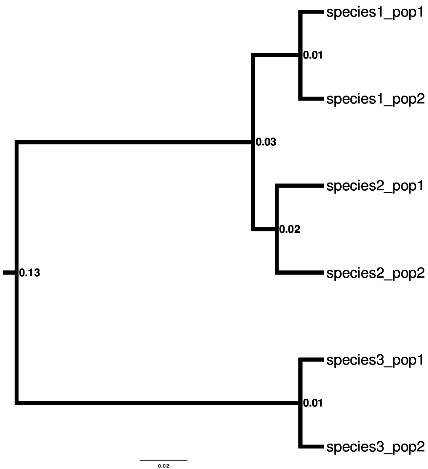
The true species tree for the three pairs of lizard populations.

So, “species-1” and “species-3” co-diverged 0.01 units (expected substitutions per site) ago, and “species-2” diverged earlier, at 0.02 units ago.

4.6.2.4. The marginal divergence time plots

We see below that under the dpp-msbayes model, the 95% HPD for the divergence time of all three species contain the true value, whereas only one of the three contain the true value under the msBayes model.

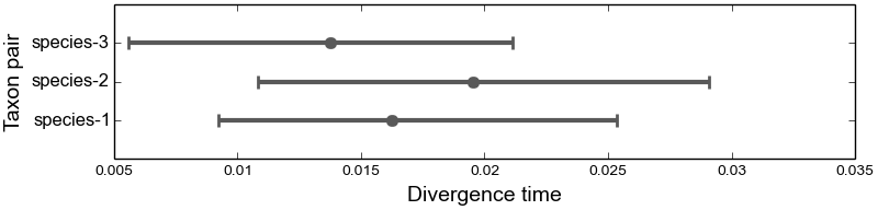
Estimated marginal divergence times under the DPP model

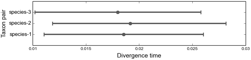
Estimated marginal divergence times under the msBayes model

4.6.2.5. The number of divergence events plots

The dpp-msbayes model correctly estimates that there were two events, but with quite a bit of uncertainty (see plot below.) The msBayes model is quite confident that there was a single divergence event, and actually has support against the correct answer of two events (negative 2ln(Bayes factor)) (see plot below.)

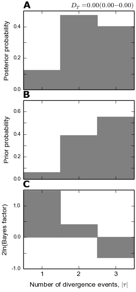
Posterior probabilities of the number of divergence events under the DPP model

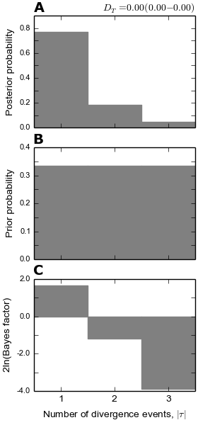
Posterior probabilities of the number of divergence events under the msBayes model

Note

Despite inferring multiple divergence events, the dispersion index of divergence times (; or “omega” in msBayes literature) is estimated to be zero. This is a great example of how “omega” is extremely sensitive to the scale of the divergence times and is not a very useful measure of “simultaneous divergence”.

4.6.2.6. The divergence models plot

The plots of the divergence models below show that both the dpp-msbayes and msBayes model infers the wrong divergence model. The dpp-msbayes weakly supports the most general divergence model with three divergence events, whereas the msBayes model quite strongly supports the model with a single divergence event. The second most probable divergence model under both analyses is the correct model; the dpp-msbayes model approximates a larger posterior probability for the correct model (0.201 vs 0.078). We can use, dmc_posterior_probs.py to determine the support for the correct divergence-time scenario under both models, which we do in the next section.

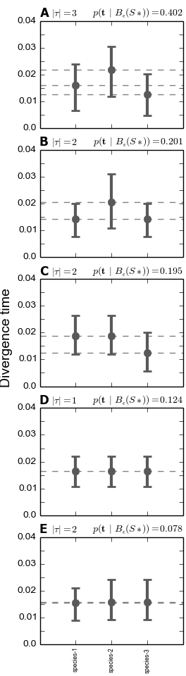
Posterior probabilities of the divergence models under the DPP model

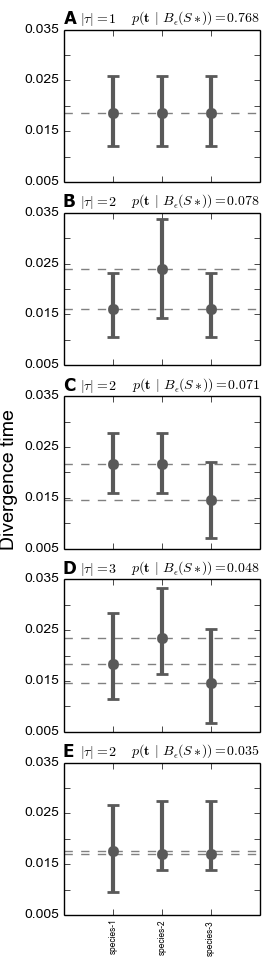
Posterior probabilities of the divergence models under the msBayes model

4.6.3. Summarzing results about divergence-time scenarios

So, we know the correct divergence-time scenario is “species-1 == species-3 < species-2”, so let’s compare the support for this divergence model under the dpp-msbayes and msBayes model:

$ dmc_posterior_probs.py -e "0 == 2 < 1" -n 10000 \
    ../../../../configs/dpp-simple.cfg \
    pymsbayes-output/d1/m1/d1-m1-s1-10000000-posterior-sample.txt.gz

Here, the -e "0 == 2 < 1" argument is the true divergence scenario we are interested in, where “0 = species-1”, “1 = species-2”, and “2 = species-3” are the indices of the taxa in the order they appear in the configuration file. The -n 10000 argument tells the program to perform 10000 simulations to estimate the prior probability of the scenario (to allow Bayes factors to be calculated). The second to last argument is the path to the configuration file that specifies the dpp-msbayes model. The last option is the path to the approximate posterior sample from the analysis under the dpp-msbayes models specified in the configuration file. This posterior-sample file is gzipped, but that’s okay, because PyMsBayes can handle gzipped files just fine.

Here is the output:

l[0] == l[2] < l[1] --- species-1 == species-3 < species-2:
-----------------------------------------------------------
posterior probability = 0.184
prior probability = 0.066
Bayes factor = 3.19102792632
2ln(Bayes factor) = 2.32068619769

Let’s do the same thing for the msBayes model:

$ dmc_posterior_probs.py -e "0 == 2 < 1" -n 10000 \
    ../../../../configs/msbayes.cfg \
    pymsbayes-output/d1/m2/d1-m2-s1-10000000-posterior-sample.txt.gz

Notice, in the last argument (the path to the posterior sample), we are using “m2” in instead of “m1” to specify the posterior sample from the analysis under the msBayes model specified in msbayes.cfg. Here is the output:

l[0] == l[2] < l[1] --- species-1 == species-3 < species-2:
-----------------------------------------------------------
posterior probability = 0.071
prior probability = 0.0764
Bayes factor = 0.923917515315
2ln(Bayes factor) = -0.158264960929

As we can see, the dpp-msbayes model approximates moderate support (2ln(BF) = 2.32) for the correct model of divergence, whereas the msBayes model actually results in support against the correct divergence model (2ln(BF) = -0.16).