4.7. A Simulation-based Validation Analysis

For this tutorial, I will assume that you have already run through the simple empirical analysis, and multi-model empirical analysis so we will go into a lot less detail here.

4.7.1. Background

As shown by [10], [9], and [8], it can be very informative to see how a model performs when applied to data where there is no shared divergences (i.e., the divergences across the taxa are independent and completely random). For example, if we find that dpp-msbayes and/or msBayes cannot reliably detect random variation in divergence times over the time scale in which we are interested, then we know that we should not interpret estimates of co-divergence by the method biogeographically (because we were likely to infer co-divergence even if the taxa diverged randomly over the period of time we are interested in).

dmc.py allows us to assess the performance of models under a wide variety of condtions very easily. All we have to do is designate configuration files with the -o option that specify models under which we want to simulate datasets; these simulated datasets will all be analyzed under the model(s) specified in the configuration files designated with the -p option.

4.7.2. The example configs for simulated datasets

If you look in the pymsbayes-tutorial-data/lizards/configs/simulated-data-configs directory within the tutorial data that you downloaded, you will see that there are three more configuration files:

• exponential-02.cfg
• exponential-04.cfg
• exponential-06.cfg

The preamble of the exponential-02.cfg file looks like:

thetaShape = 4.0
thetaScale = 0.001
ancestralThetaShape = 0
ancestralThetaScale = 0
thetaParameters = 000
tauShape = 1.0
tauScale = 0.02
timeInSubsPerSite = 1
bottleProportionShapeA = 0
bottleProportionShapeB = 0
bottleProportionShared = 0
migrationShape = 0
migrationScale = 0
numTauClasses = 3

The setting numTauClasses = 3 will constrain the model to only sample from the most general model of divergence with three divergence-time parameters (one for each species). Thus, under this model the three pairs of populations diverge randomly according to the prior on divergence time (tauShape = 1.0; tauScale=0.02), which is an exponential distribution with a mean of 0.02. The configuration files exponential-04.cfg and exponential-06.cfg are identical except that their exponential distribution on divergence times have means of 0.04 and 0.06, respectively.

4.7.3. Running the simulation-based analysis

We can use dmc.py to generate as many datasets as we wish under each of these three models (random divergence times from an exponential distribution with a mean of 0.02, 0.04, and 0.06), and analyze all of the simulated datasets under the same two models we used to analyze the lizard data.

If we are in the pymsbayes-tutorial-data/lizards/configs, all we have to do is:

$ dmc.py -o simulated-data-configs/exponential-02.cfg \
    simulated-data-configs/exponential-04.cfg \
    simulated-data-configs/exponential-06.cfg \
    -p dpp-simple.cfg msbayes.cfg \
    -r 100 -n 5000 --no-global-estimate

The -r 100 option specifies to simulate 100 datasets under each of the three models specified in the configuration files listed after the -o flag, and analyze them all under the models specified in the configuration files listed after the -p flag. To keep the runtime short, we also specify with the -n 5000 that only 5000 samples will be sampled for each of the prior models (dpp-simple.cfg and msbayes.cfg). We also specify not to perform model-averaging analyses on the 300 simulated datasets by using the --no-global-estimate option; there is no reason you cannot perform model-averaging analyses, but it will save a little bit of time in this trivial example.

NOTE, the results of this example analysis will not be meaningful, because 5000 samples from the prior models are not sufficient for a meaningful approximation of the posterior. The command above took less than 3 minutes to run on my laptop.

After running this example simulation-based analysis you should have a new pymsbayes-results directory within the pymsbayes-tutorial-data/lizards/configs/simulated-data-configs (by default dmc.py puts the results directory in the same directory as the first “observed config file” specified with the -o option).

4.7.4. The output

The output of a simulation-based analysis has the same structure and is very similar to the empirical analyses you have already run. One difference is that the pymsbayes-results/observed-summary-stats now has three files (observed-1.txt, observed-2.txt, and observed-3.txt), which each contain the “observed” summary statistics from 100 simulated datasets.

Also, the data-model-key file pymsbayes-results/pymsbayes-output/data-key.txt now has three keys (“d1”, “d2”, and “d3”) which correspond to the observed-summary-stats files. Furthermore, the pymsbayes-info.txt file tells us that the “1”, “2”, and “3” correspond with the configuration files exponential-02.cfg, exponential-04.cfg, and exponential-06.cfg, respectively.

From this, we know, for example, that all of the results in pymsbayes-results/pymsbayes-output/d3/m2/ directory are from datasets simulated under the d3 model (exponential-06.cfg) and analyzed under the m2 model (msbayes.cfg). You will also see that there are results for 100 simulated datasets in that directory (i.e., you will see file prefixes from d3-m2-s1 to d3-m2-s100).

Overall, you will find that there are results for all the data models analyzed under all of the prior models nested in the directories:

• d1/m1/
• d1/m2/
• d2/m1/
• d2/m2/
• d3/m1/
• d3/m2/

And, for each of these, there are results for 100 simulated datasets.

4.7.5. Summarizing the results

To summarize the results across the 100 simulated datasets across all 6 directories of simulation results, we can use the dmc_sum_sims.py program. All we need to do is tell dmc_sum_sims.py where to find the pymsbayes-info.txt file from our analysis:

$ dmc_sum_sims.py pymsbayes-results/pymsbayes-info.txt

After running dmc_sum_sims.py we will find a compressed (gzipped) file named results.txt.gz in each of the output directories:

• d1/m1/results.txt.gz
• d1/m2/results.txt.gz
• d2/m1/results.txt.gz
• d2/m2/results.txt.gz
• d3/m1/results.txt.gz
• d3/m2/results.txt.gz

These files summarize the results across the analyses of all 100 simulated datasets. We can also tell dmc_sum_sims.py to create some plots summarizing the results:

$ dmc_sum_sims.py pymsbayes-results/pymsbayes-info.txt --plot

This will create a new directory pymsbayes-results/plots with 6 PDF files containing plots:

• dpp-simple_accuracy_cv_median.pdf
• dpp-simple_power_psi_mode.pdf
• dpp-simple_power_psi_prob.pdf
• msbayes_accuracy_cv_median.pdf
• msbayes_power_psi_mode.pdf
• msbayes_power_psi_prob.pdf

Three of the PDFs summarize the results when the simulated data were analyzed under the model specified in the dpp-simple.cfg configuration file, and thus their file names begin with dpp-simple. The other three summarize the results when the simulated data were analyzed under the model specified in msbayes.cfg, and thus their file names begin with msbayes.

Let’s take a look at the three kinds of plots that are created.

4.7.6. CV accuracy plots

These plots simply compare the true versus estimated (posterior median) values for the coefficient of variation (CV) of divergence times.

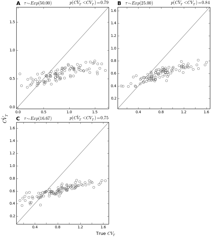
The true versus estimated values of the coefficient of variation of divergence times.

4.7.7. Histograms of the estimated number of divergence events

These plots show a histogram of the estimated (posterior mode) number of divergence events across all the analyses of simulated data.

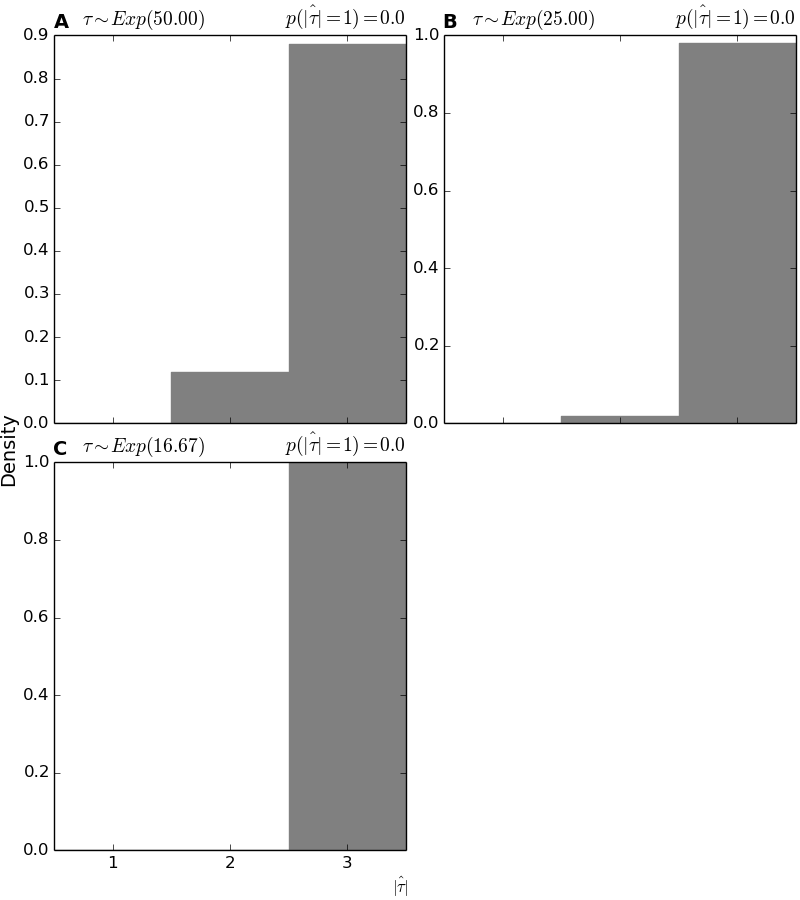
Histograms of the estimated number of divergence events.

4.7.8. Histograms of the support for the single divergence model

These plots show the histograms of the approximated posterior probability of the single-divergence-event model across all the analyses of simulated data.

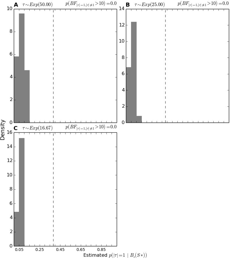
Histogram of the support (posterior probability) for the single divergence model.